Cluster Analysis in R: Hierarchical Clustering
- Martin Calvino

- Oct 24, 2021
- 7 min read
Given a dataset, cluster analysis allows for the uncovering of subgroups of observations that share common characteristics. It is a data-reduction technique because large number of observations can be reduced to a discrete number of clusters or types. A group of observations being more similar to each other relative to observations in other groups is known as a cluster [1]. Although there are various clustering approaches [2], the most widely used are hierarchical agglomerative clustering and partitioning clustering [1-4]. In this work, I will focus on hierarchical clustering.
In hierarchical clustering, each observation begins at its own cluster. Clusters are then subsequently grouped two at a time until all clusters are included within a single big cluster. The clustering algorithms used in hierarchical clustering are:
(a) single linkage > shortage distance between an observation in one cluster and an observation in another cluster
(b) complete linkage > longest distance between an observation in one cluster and an observation in another cluster
(c) average linkage > average distance between each observation in one cluster and each observation in another cluster
(d) centroid > distance between centroids (vector of variable means) of two clusters
(e) Ward > the ANOVA sum of squares between two clusters added up over all the variables
The dataset I am focusing on contains approximately 300,000 mortgage applications in the state of New Jersey for the year 2018. This dataset was previously filtered based on two ethnic groups: (1) not.hispanic; and (2) latino applicants, respectively. It was obtained from the Consumer Financial Protection Bureau's website [5] and is associated with the Home Mortgage Disclosure Act (HMDA) that requires financial institutions to disclose loan-level information about mortgages.
My objective was to apply cluster analysis to this dataset in order to uncover subgroups of observations.
This dataset contains 295,286 mortgage applications (observations) across 99 variables [6]. I am interested in the variables pertaining to the loan amount requested by the applicant and his or her reported income. Most importantly, are there distinctive subgroups of applicants based on loan amount and income when the dataset is divided according to ethnicity (not.hispanic versus latino applicants)?
Load the dataset into R:
# mortgage applications for the year 2018 as 'may18'
# load dataset
may18 <- read.csv(file.choose())

str(may18) # 295,286 observations and 99 variables
Select variables / columns of interest and create a new data frame containing those:
# select variables of interest (if variable is categorical > make it into a factor)

bank <- factor(may18$lei)
levels(bank) #805 banks

ethnicity <- factor(may18$derived_ethnicity)
levels(ethnicity) # latino and not.hispanic

race <- factor(may18$derived_race)
levels(race) # 8 race descriptions

sex <- factor(may18$derived_sex)
levels(sex) # 4 descriptions

county <- factor(may18$county_code)
levels(county) # 132 counties

action <- factor(may18$action_taken)
levels(action) # 8 actions

purpose <- factor(may18$loan_purpose)
levels(purpose) # 6 purposes

amount <- may18$loan_amount

value <- as.numeric(may18$property_value) # was encoded as "string" in dataset

income <- 1000*may18$income

denial <- factor(may18$denial_reason.2)
levels(denial)

reduced.may18 <- data.frame(bank, ethnicity, race, sex, county, action, purpose, amount, value, income, denial)

head(reduced.may18)
Identify and visualize missing values (NAs) from dataset using the VIM library [7]:
# identify missing values
# because is.na() returns TRUE if a missing value (NA) is present;
# and because TRUE=1 and FALSE=0 then you can add all TRUES using
the sum() and mean() functions

sum(is.na(reduced.may18)) # 365,339 missing values (NAs)

mean(is.na(reduced.may18)) # 0.1124762 ~ 11.2% of values in
reduced.may18 dataset are missing values

# let's visualize the missing values

install.packages("VIM", dependencies=TRUE)
library("VIM")

# the aggr() function depicts the missing values (in counts or percentage) for each variable alone or in combination with each other

aggr(reduced.may18, prop=FALSE, numbers=TRUE)


# the matrixplot() function depicts missing data (in red) for each observation in the data frame
# values for each variable are rescaled to the interval [0,1] and represented by grey colors (lighter colors > lower values / darker colors > higher values)

matrixplot(reduced.may18)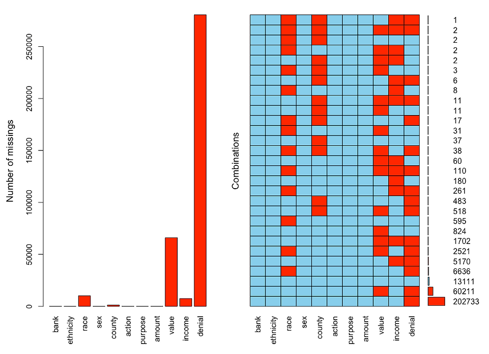
Figure 1. Output of the aggr( ) function from the VIM package visualizing missing values (shown in red) for each variable in the dataset (left panel), and for the combination of variables (right panel).
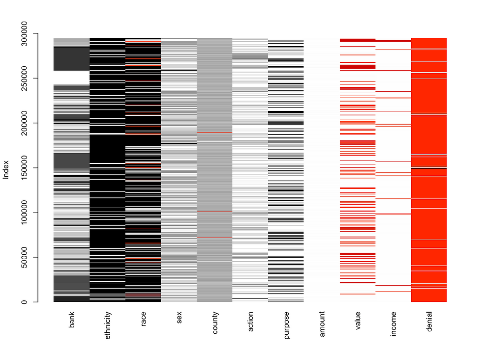
Figure 2A. Output of the matrixplot( ) function from the VIM package visualizing missing values for each (and all) observations / loan applications in the dataset. Missing values are shown in red, whereas all other values are scaled between 0 to 1 and colored in gray scale: lower values are lighter whereas higher values are darker.
Remove missing values from dataset and 'discard' the denial variable because it has a great amount of missing values:
# re-create reduced.may18 without denial variable because it has so many missing values

reduced.may18 <- data.frame(bank, ethnicity, race, sex, county, action, purpose, amount, value, income)

head(reduced.may18)

# remove missing values

reduced.may18 <- na.omit(reduced.may18)
str(reduced.may18) # 215,844 observations and 10 variables
head(reduced.may18)

# visually confirm missing values are gone

matrixplot(reduced.may18)
Figure 2B. Output of the matrixplot( ) function from the VIM package after all missing values were removed with na.omit( ) function and the variable denial was discarded.
Because loan applications in 2018 from not.hispanic applicants (193,179 applications) greatly superseded those from latinos (22,665 applications) , I created two new datasets containing 10,000 applications each (one dataset for not.hispanic and the other for latino applicants, respectively).
# filter reduced.may18 based on ethnicity (Not.Hispanic) using grep() function

not.hispanic <- reduced.may18[grep("Not.Hispanic", reduced.may18$ethnicity), ]

str(not.hispanic) # data frame containing 193,179 observations and 10 variables

# filter may18 based on ethnicity (Latino) using grep() function

latino <- reduced.may18[grep("Latino", reduced.may18$ethnicity), ]
str(latino) # 22,665 observations and 10 variables


# sample the same number of observations (10,000) for each filtered dataset (not.hispanic and latino)

not.hispanic.sampled <- not.hispanic[sample(1:nrow(not.hispanic), 10000, replace=FALSE), ]

latino.sampled <- latino[sample(1:nrow(latino), 10000, replace=FALSE), ]
Inspect the summary statistics for not.hispanic and latino datasets:
# let's inspect these 'sampled' dataframes

summary(not.hispanic.sampled)
summary(latino.sampled)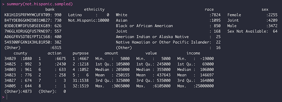
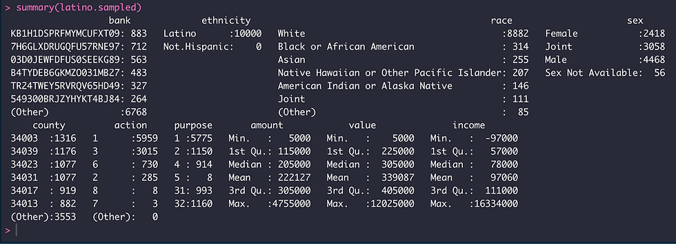
We can see that the top 5 banks receiving loan applications during 2018 are the same (but ranked differently) for not.hispanic and latino applicants with the exception of PNC Bank in not.hispanic dataset and Santander for the latino dataset. The race composition differed among datasets as well, with white and Asian races being the top two for not.hispanic applicants relative to white and black or African American for latino applicants. The top three counties also differed for each group of applicants in New Jersey; Ocean, Monmouth and Bergen for not.hispanic and Bergen, Union and Middlesex for latinos. The median income from not. hispanic applicants was $106,000 relative to $78,000 for latinos although the median for loan amounts and property values were similar.
I will perform hierarchical clustering ONLY with numeric variables since I want to scale the data prior to calculating distances. For hierarchical clustering with categorical variables, refer [4].
# let's take only numeric variables so I can scale the data prior to the calculation of distance

not.hispanic.sampled.numeric <- data.frame(not.hispanic.sampled$amount, not.hispanic.sampled$value,
not.hispanic.sampled$income)

head(not.hispanic.sampled.numeric)

latino.sampled.numeric <- data.frame(latino.sampled$amount, latino.sampled$value, latino.sampled$income)

head(latino.sampled.numeric)

# scale data > standarize variables > [x-mean(x) / sd(x)]

not.hispanic.scaled <- scale(not.hispanic.sampled.numeric)

latino.scaled <- scale(latino.sampled.numeric)

head(not.hispanic.scaled)

head(latino.scaled)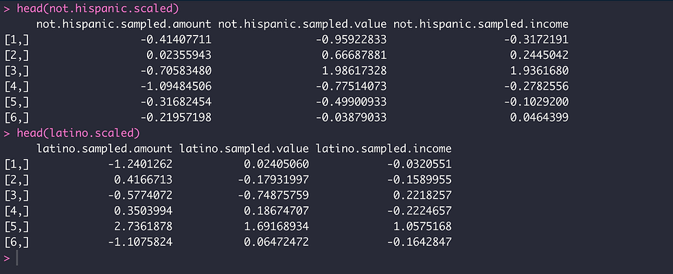
With the data scaled, I am now in a position to infer the best number of clusters to be used as k in hierarchical clustering. I can accomplish this using the NbClust package [8]; this package provides indices for estimating the best number of clusters in a cluster analysis.
# determine the best number of clusters

library("NbClust")

nc.not.hispanic <- NbClust(not.hispanic.scaled[1:1000,], distance="canberra", min.nc=2, max.nc=15, method="ward.D2")

table(nc.not.hispanic$Best.n[1,]) # best number of clusters is 3

nc.latino.scaled <- NbClust(latino.scaled[1:1000,], distance="canberra", min.nc=2, max.nc=15, method="ward.D2")

table(nc.latino.scaled$Best.n[1,]) # best number of clusters is 2
Using NbClust I obtained an estimation of 3 clusters for the dataset containing not.hispanic applicants; and 2 clusters for the dataset containing latino loan applicants.
Calculate distance matrices and determine clusters:
# calculate distance: not.hispanic
d.not.hispanic <- dist(not.hispanic.scaled, method="canberra")

# calculate clusters: not.hispanic
hc.d.not.hispanic <- hclust(d.not.hispanic, method="ward.D2")

# assign number of clusters to observations: not.hispanic
not.hispanic.cluster_assignments <- cutree(hc.d.not.hispanic, k=3)

table(cluster_assignments)
# cluster 1 = 4,747 observations
# cluster 2 = 1,825 observations
# cluster 3 = 3,428 observations

# calculate distance: latino
d.latino <- dist(latino.scaled, method="canberra")

# calculate clusters: latinos
hc.d.latino <- hclust(d.latino, method="ward.D2")

# assign number of clusters to observations: latino
latino.cluster_assignments <- cutree(hc.d.latino, k=2)

table(latino.cluster_assignments)
# cluster 1 = 5528 observations
# cluster 2 = 4472 observations
Add cluster assignments to not.hispanic and latino data frames and plot the results:
library("dplyr")

not.hispanic.clustered <- mutate(not.hispanic.sampled.numeric, cluster=not.hispanic.cluster_assignments) # add cluster assignments to dataframe

head(not.hispanic.clustered)

latino.clustered <- mutate(latino.sampled.numeric, cluster=latino.cluster_assignments) #add cluster assignments to dataframe

head(latino.clustered)

# plot and color data point based on cluster assignments

library("ggplot2")

ggplot(not.hispanic.clustered, aes(x=not.hispanic.sampled.amount, y=not.hispanic.sampled.income, color=factor(cluster))) + geom_point(size=0.35, position="jitter", alpha=0.6) + coord_cartesian(xlim=c(0, 1000000), ylim=c(0, 500000))

ggplot(latino.clustered, aes(x=latino.sampled.amount, y=latino.sampled.income, color=factor(cluster))) + geom_point(size=0.35, position="jitter", alpha=0.6) + coord_cartesian(xlim=c(0, 1000000), ylim=c(0, 500000))
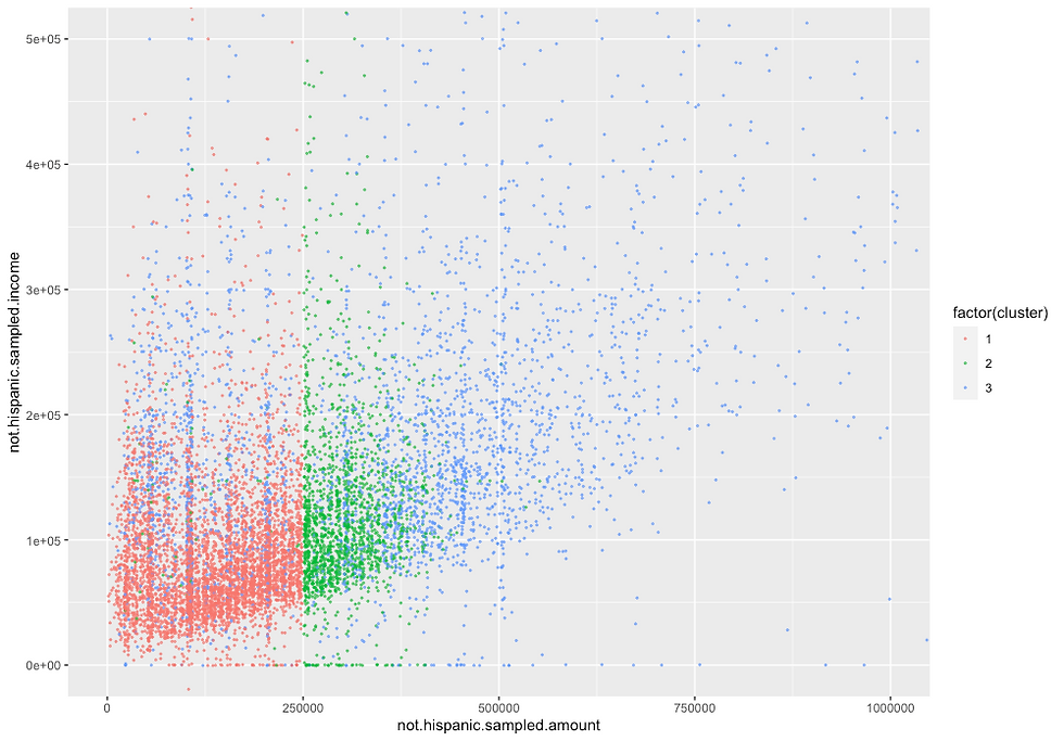
Figure 3A. Plot depicting the relationship between the loan amount requested versus the income reported for not.hispanic applicants. Data points are colored based on cluster assignments.
In the graph above, we can see that hierarchical agglomerative clustering have uncovered three distinct subgroups of not.hispanic applicants. The first group/cluster (colored in red) is composed of not.hispanic applicants that requested loan amounts up to $250,000 and reported annual income up to $150,000. The second group of applicants (colored in green) requested loan amounts up to $375,000 and reported annual income up to $300,000. The third group of applicants (colored in blue) is not as well defined as the first two groups, requesting loan amounts up to $1M and reported income up to $500,000.

Figure 3B. Plot depicting the relationship between the loan amount requested versus the income reported for latino applicants. Data points are colored based on cluster assignments.
In the graph above, we can see that hierarchical agglomerative clustering have uncovered two distinct subgroups of latino applicants. The first group/cluster (colored in red) is composed of latino applicants that requested loan amounts below $250,000 and reported annual income primarily below $100,000. The second group of applicants (colored in green) requested loan amounts primarily up to $500,000 and reported annual income primarily below $150,000.
We can have a more specific understanding of applicants for each cluster when we look at the statistics of not.hispanic and latino applicants:
# analyze stats for each cluster

aggregate(not.hispanic.clustered, by=list(cluster=not.hispanic.clustered$cluster), median)

aggregate(latino.clustered, by=list(cluster=latino.clustered$cluster), median)

Above we can see the median values for loan amount requested and reported income for each subgroup/cluster of not.hispanic applicants. These values differed from those for latino applicants as we can see below:

Finally, we can visualize the clustering of applicants in a dendrogram:
install.packages("dendextend", dependencies=TRUE)

library("dendextend")

# not.hispanic dendrogram
dend.not.hispanic <- as.dendrogram(hc.d.not.hispanic)

colored.dend.not.hispanic <- color_branches(dend.not.hispanic, k=3)

plot(colored.dend.not.hispanic, hang=-1, cex=0.1, pin=c(11,9))

# latino dendrogram
dend.latino <- as.dendrogram(hc.d.latino)

colored.dend.latino <- color_branches(dend.latino, k=2)

plot(colored.dend.latino, hang=-1, cex=0.1, pin=c(11,9))
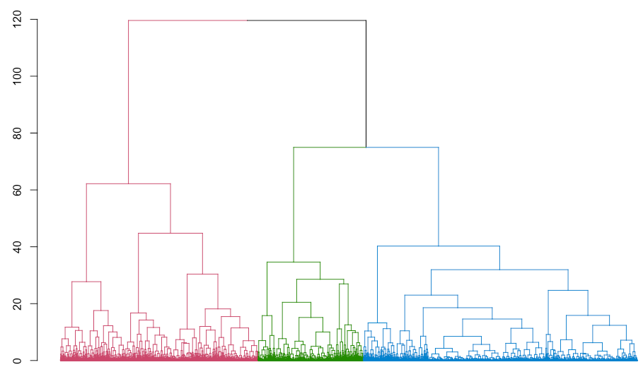
Figure 4A. Dendrogram displaying the agglomerative hierarchical clustering of 10,000 not.hispanic loan applicants during 2018 in New Jersey. Cluster assignments are colored as in Figure 3A. Scale for the y-axis shows distance measures.
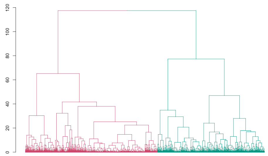
Figure 4B. Dendrogram displaying the agglomerative hierarchical clustering of 10,000 latino loan applicants during 2018 in New Jersey. Cluster assignments are colored as in Figure 3B. Scale for the y-axis shows distance measures.
In summary, agglomerative hierarchical clustering proved to be a valuable method for uncovering subgroups of loan applicants for not.hispanic and latino population in New Jersey during 2018. This approach worked well when considering numeric variables from the datasets. I've previously tried this approach with categorical variables of interest without obtaining a satisfactory and/or convincing result.
REFERENCES
[1] Robert L. Kabacoff (2015). R in action: data analysis and graphics with R (Second Edition). Published by Manning, Shelter Island, New York.
[2] Sunit Prasad (2020). Different types of clustering methods and applications. URL: https://www.analytixlabs.co.in/blog/types-of-clustering-algorithms/ Accessed October 20, 2021.
[3] Dmitry Gorenshteyn course on Datacamp: Cluster Analysis in R. URL: https://www.datacamp.com Accessed October 20, 2021.
[4] Anastasia Reusova (2018). Hierarchical clustering on categorical data in R. Published on Towards Data Science. URL: https://towardsdatascience.com/hierarchical-clustering-on-categorical-data-in-r-a27e578f2995 Accessed on October 23, 2021.


Comments