Mapping geographic data in R: home loan applications per county
- Martin Calvino

- Dec 31, 2022
- 5 min read
Updated: Jan 2, 2023
As part of my ongoing project on the analysis and visualization of home loans --available as part of the Home Mortgage Disclosure Act (HMDA) dataset -- with emphasis on latino applicants from New Jersey, I now describe here the mapping of such data on a geographical scale. I focused my attention on the percentage of denied loans per county at the state level as well as the national level.
In the approach shown here, I used the packages sf for working with geodata, and ggplot2 for visualization. The sf package depends on a library named GDAL (Geospatial Data Abstraction Library) and you need to install it prior to sf.
To load geographic boundaries in R, I used the package rnaturalearth. I followed the tutorial "Mapping Geographic Data in R" published in the FlowingData website, and modified the code according to my needs, writing my own code as well in order to obtain the desired outcomes.
The approach I took consisted on four sections:
Section A > home loan data wrangling
Section B > load geographic data to display counties
Section C > incorporate home loan data into county geographic data
Section D > visualize home loan data on map of United States
I first describe my analysis on a nationwide scale, followed by mapping home loan data at the state (New Jersey) level.
Home Loan Data Wrangling (Section A)
I downloaded from the Consumer Financial Protection Bureau (CFPB) website a dataset on home loans for the year 2021 at the nationwide level, sorted on the ethnicity of the home loan applicant (latino vs. not.latino). This dataset consisted of:
19,182,225 loan applications (2,330,524 latino applicants + 16,851,701 not.latino applicants)
4,333 financial institutions
The key aspect of this section was to obtain the percentage of denied loans per county for each group of applicants (latino vs. not.latino).
# SECTION A > home loan data wrangling

# load datasets
# all banks nationwide 2021 as 'aban21'
aban21 <- read.csv(file.choose())

# inspect variable names
colnames(aban21)

# select variables of interest (voi)
county <- aban21$county_code
ethnicity <- aban21$derived_ethnicity
action <- aban21$action_taken

# create new data frame
aban21.voi <- data.frame(county, ethnicity, action)

# remove missing values
aban21.voi <- na.omit(aban21.voi) # 18,970,270 observations
head(aban21.voi, n = 25)

# recode ethnicity
aban21.voi$ethnicity[aban21.voi$ethnicity == "Hispanic or Latino"] <- "Latino"
aban21.voi$ethnicity[aban21.voi$ethnicity == "Not Hispanic or Latino"] <- "Not.Latino"

# arrange observations by county
aban21.voi <- arrange(aban21.voi, county)
head(aban21.voi, n = 25)

# is there home loan data for how many counties?
COunties <- factor(aban21.voi$county)
length(levels(COunties)) # 3,222 counties
View(COunties)

# partition aban21.voi into 2 data frames based on ethnicity
# each data frame will lead to two maps

# latino data frame
latino.df <- filter(aban21.voi, ethnicity == "Latino")
# not.latino data frame
not.latino.df <- filter(aban21.voi, ethnicity == "Not.Latino")

# count loans per county for latinos' applicants
latino.loans.per.county <- latino.df %>%
  group_by(county) %>%
  tally()

View(latino.loans.per.county) # financial institutions in 3,086 counties processed loan applications from latinos

# count loans per county for not.latinos' applicants
not.latinos.per.county <- not.latino.df %>%
  group_by(county) %>%
  tally()

View(not.latinos.per.county) # financial institutions in 3,203 counties processed loan applications from not.latinos

# NOW... select denied applications for both latinos and not.latinos and count how may applications there are per county
latinos.denied <- filter(latino.df, action == 3 | action == 7)
not.latinos.denied <- filter(not.latino.df, action == 3 | action == 7)

# count denied loans per county for latinos' applicants
denied.latino.loans.per.county <- latinos.denied %>%
  group_by(county) %>%
  tally()
View(denied.latino.loans.per.county)

# count denied loans per county for not.latinos' applicants
denied.not.latinos.per.county <- not.latinos.denied %>%
  group_by(county) %>%
  tally()
View(denied.not.latinos.per.county)

# implement join operation to combine latino.loans.per.county with denied.latinos.loans.per.county
j1.latino.per.county <- latino.loans.per.county %>%
  left_join(denied.latino.loans.per.county, by = "county")

View(j1.latino.per.county)

# rename variables
names(j1.latino.per.county)[2] <- "all.loans"
names(j1.latino.per.county)[3] <- "denied.loans"
View(j1.latino.per.county)

# calculate percentage of loans that were denied for each county
j1.latino.per.county <- mutate(j1.latino.per.county, pct.denied = (denied.loans*100)/all.loans)
View(j1.latino.per.county)


# implement join operation to combine not.latinos.per.county with denied.not.latinos.per.county
j2.not.latinos.per.county <- not.latinos.per.county %>%
  left_join(denied.not.latinos.per.county, by = "county")

View(j2.not.latinos.per.county)

# rename variables
names(j2.not.latinos.per.county)[2] <- "all.loans"
names(j2.not.latinos.per.county)[3] <- "denied.loans"
View(j2.not.latinos.per.county)

# calculate percentage of loans that were denied for each county
j2.not.latinos.per.county <- mutate(j2.not.latinos.per.county, pct.denied = (denied.loans*100)/all.loans)
View(j2.not.latinos.per.county)
The resulting data frames are as shown below for not.latino applicants (left image) and latinos (right image), respectively.
I now have the percentage of denied loans per county for each ethnic group of loan applicants. The next step is to incorporate this data into the shape files containing the necessary information to draw county boundaries, so they ultimately can be color-filled with percentage of denied loans data.
# SECTION B > load geographic data to display counties

# load the grographical data

# locate ne_10m_admin_2_counties.shp loaded from Natural Earth:
# https://www.naturalearthdata.com/downloads/10m-cultural-vectors/10m-admin-2-counties/
counties.file <- file.choose()
counties.file # "/home/calviot/Desktop/ne_10m_admin_2_counties.shp"

# read file with read_sf
counties <- read_sf(counties.file)
print(counties, n=0)
View(counties)

# get CRS details of counties
st_crs(counties)

# EPSG codes of different coordinate systems can be retrieved from https://epsg.io/
# You use the EPSG code to specify the CRS to use in the coord_sf() function.
# counties = st_set_crs(counties, "EPSG:4326) # set CRS

# reorder rows based on county codes
counties <- arrange(counties, CODE_LOCAL) # county codes start with 0 in CODE_LOCAL
counties
I now join the loan data with the geographic data for counties:
# SECTION C > incorporate home loan data into county geography data


# add leading 0s to county codes in home loan datasets and rename the variable CODE_LOCAL so I can perform left_join() operation
j2.not.latinos.per.county$county[1:316] <- paste0("0", j2.not.latinos.per.county$county) # add leading 0 only until row 316
names(j2.not.latinos.per.county)[1] <- "CODE_LOCAL"
names(j2.not.latinos.per.county)[4] <- "pct.denied.NOT.latinos"
View(j2.not.latinos.per.county)
# keep only COUNTY_CODE and pct.denied.NOT.latinos variables
j2 <- j2.not.latinos.per.county[, -c(2,3)]
View(j2) # great!

j1.latino.per.county$county[1:256] <- paste0("0", j1.latino.per.county$county) # add leading 0 only until row 256
names(j1.latino.per.county)[1] <- "CODE_LOCAL"
names(j1.latino.per.county)[4] <- "pct.denied.latinos"
View(j1.latino.per.county)
# keep only COUNTY_CODE and pct.denied.latinos variables
j1 <- j1.latino.per.county[, -c(2,3)]
View(j1) # great!

# join j2 with j1
j21 <- j2 %>%
  left_join(j1, by = "CODE_LOCAL")
View(j21) # super


# add a column with percentage difference in denials between not.latinos and latinos
j21 <- mutate(j21, pct.diff =  pct.denied.latinos - pct.denied.NOT.latinos)
View(j21) # super duper
summary(j21)


# incorporate loan data into county geography data
counties.loanData.WF <- counties %>%
  left_join(j21, by = "CODE_LOCAL")
View(counties.loanData.WF)
And now I can create the choropleth map with the fill aesthetic mapped to percentage of denied loans for each ethnic group.
# SECTION D > visualize home loan data on map of the US (partitioned by county)

# not.latinos loan applicants
counties.loanData.WF <- mutate(counties.loanData.WF, pct.diff_category = cut(pct.denied.NOT.latinos, breaks = c(1, 5, 10, 15, 20, 25, 100)))

map <- ggplot(counties.loanData.WF, aes(fill = pct.diff_category)) +
  geom_sf(color = "white", size = 0.1) +
  scale_fill_brewer(palette = "Blues", name = "pct.diff per county",
                    labels = c("1-5", "6-10", "11-15", "16-20", "21-25", "26% or more")) +
  theme_minimal()

map %+%
  filter(counties.loanData.WF, REGION != "AK", REGION != "HI")

# latino loan applicants
counties.loanData.WF <- mutate(counties.loanData.WF, pct.diff_category = cut(pct.denied.latinos, breaks = c(1, 5, 10, 15, 20, 25, 100)))

map <- ggplot(counties.loanData.WF, aes(fill = pct.diff_category)) +
  geom_sf(color = "white", size = 0.1) +
  scale_fill_brewer(palette = "Blues", name = "pct.diff per county",
                    labels = c("1-5", "6-10", "11-15", "16-20", "21-25", "26% or more")) +
  theme_minimal()

map %+%
  filter(counties.loanData.WF, REGION != "AK", REGION != "HI")
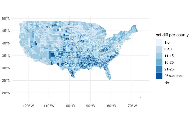
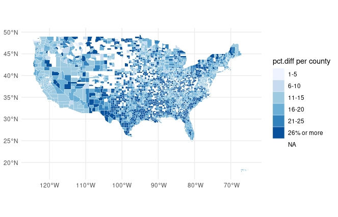
The resulting maps are shown below for not.latino loan applicants (left image) and latinos (right image) respectively.

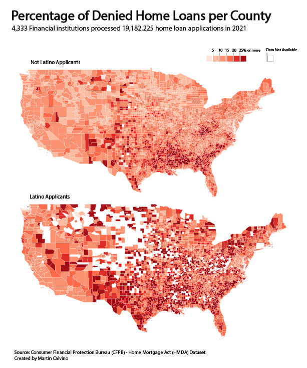
We can see above that for not.latino applicants, loans were denied in higher percentages primarily on counties in southern states such as Arkansas, Louisiana, Mississippi, Alabama and Georgia and South Carolina; and also in Kentucky.

Whereas for latino loan applicants, applications were denied primarily on counties belonging to the following states: New Mexico - Texas - Arkansas - Louisiana - Mississippi - Alabama - Georgia - South Carolina - Pennsylvania - New York - Vermont and Maine. We can also see there are many more counties colored dark blue, indicating higher percentage of denied loans compared to not.latino applicants. Nationwide, the media value for percentage of denied loans was 18.5% for latinos compared to 13.5% for not.latino applicants.
After changing the fill aesthetic to orange and exporting the graphs as .svg files, I could import them into Adobe Illustrator and re-work the visualization for better understanding and presentation.


Comments