Logistic Regression, Contingency Tables, Tests of Independence & Summary Statistics in R
- Martin Calvino

- Jun 7, 2022
- 14 min read
I continue my work on using R to explore data containing home mortgage applications in the state of New Jersey for the years 2018, 2019 and 2020, respectively. I obtained these three datasets from the Consumer Financial Protection Bureau's website. They are associated with the Home Mortgage Disclosure Act (HMDA) that requires financial institutions to disclose loan-level information about mortgages. I am interested in examining the relation between the ethnicity (latino vs not.hispanic) of the home loan applicant with the rest of the variables present in the dataset.
To access my previous work on the HMDA dataset please refer to:
Exploratory Data Analysis > weblink here
Principal Component Analysis > weblink here
Hierarchical Clustering > weblink here
In this post I will employ a battery of data science approaches to uncover new insights on banking practices relating to home loan applications, with an emphasis on applications from latinos living in New Jersey. The computational approaches I employed were guided by concrete questions I wanted to answer.
Question 1
Is the applicant's ethnicity (latino vs not.hispanic) a contributing factor in the decision of the bank in accepting or denying a home loan?
The above question can be answered by the implementation of regression, a set of methods in which a response variable (also known as dependent or outcome variable) is predicted from one or several predictor variables (also known as independent or explanatory variables). Regression analysis is often used to identify the explanatory variables influencing the outcome variable. Logistic regression is a particular type of regression analysis in which the outcome variable is categorical (binary) whereas the explanatory variables are quantitative and/or categorical. By categorizing home loan applications in two groups (loan originated vs loan denied) based on the action taken by the bank, I can use logistic regression to address the relation between the ethnicity of the applicant and the odds of the loan being approved or denied.
In R, logistic regression is implemented with the glm() function. Prior to this, I need to prepare the data in a format that is amenable to my purpose.
# load libraries needed
library(tidyverse)
library(psych)
library(gplots)
library(vcd)
library(graphics)

# import HMDA datasets (2018-2019-2020)
d18 <- read.csv(file.choose()) # 295,286 observations x 99 variables year 2018
d19 <- read.csv(file.choose()) # 335,661 observations x 99 variables year 2019
d20 <- read.csv(file.choose()) # 486,304 observations x 99 variables year 2020

# join datasets using rbind() which adds rows to a data frame
dA <- rbind(d18, d19, d20) # 1,117,251 observations x 99 variables

# inspect data frame
View(dA)

# select variables of interest from dA data frame and rename them for simplicity
year <- dA$activity_year
bank <- dA$lei
ethnicity <- dA$derived_ethnicity
race <- dA$derived_race
action <- dA$action_taken
loanA <- dA$loan_amount
ltv <- as.numeric(dA$loan_to_value_ratio)
ir <- as.numeric(dA$interest_rate)
pv <- as.numeric(dA$property_value)
inc <- (dA$income)*1000
houseAge <- dA$tract_median_age_of_housing_units

# create new data frame dB with variables of interest
dB <- data.frame(year, bank, ethnicity, race, action, loanA, ltv, ir, pv, inc, houseAge)
str(dB)

# keep observations/rows/applications coming from applicants self-identified in one of the three major races: Asian, Black or African American and White
dB <- dB[dB$race == "White" | dB$race == "Black or African American" | dB$race == "Asian", ] # 1,058,084 observations x 11 variables

# visualize outliers for numeric columns/variables
boxplot(dB[, c(6:11)]) # plotA
boxplot(dB[, 11]) # there is no outliers for houseAge

# EXAMPLE: visualize and remove outliers for one variable (example column 6 that is loanA variable)
# outliers.dB.loanA <- boxplot(dB[, 6])$out
# dB <- dB[-which(dB[, 6] %in% outliers.dB.loanA), ]
# boxplot(dB[, 6])

# since I need to do the above for the other numeric variables (in dB except for houseAge) I write a custom function for the task
discard.Outliers <- function(db, dataSet.Variables) {
  outlier <- boxplot(dataSet.Variables)$out
  db.oo <- db[-which(dataSet.Variables %in% outlier), ]
  return(db.oo)
}

# remove outliers one variable at a time
dB.6 <- discard.Outliers(dB, dB[, 6])
dB.7 <- discard.Outliers(dB.6, dB.6[, 7])
dB.8 <- discard.Outliers(dB.7, dB.7[, 8])
dB.9 <- discard.Outliers(dB.8, dB.8[, 9])
dB.10 <- discard.Outliers(dB.9, dB.9[, 10])

boxplot(dB.10[, c(6:11)]) # inspect that outliers were effectively removed

describe(dB.10) # the income variable has observations with negative values that need to be removed

# remove negative values from the income variable
dB.10 <- dB.10[dB.10$inc > 0, ]

boxplot(dB.10[, c(6:11)]) # plotB
# ^ compare plotA with plotB and see how outliers were removed from numeric values and how observations with negative income values were removed

# rename dB.10 dataframe to dB.curated
dB.curated <- dB.10 # 899,298 observations x 11 variables
describe(dB.curated[, c(6:11)])


# select observations/rows/applications whose value for the variable action (action taken by the bank on the loan application) ...
# ... relates to 'loan originated' (action == 1) and "loan denied" (action == 3)
dB.load <- dB.curated[dB.curated$action == 1 | dB.curated$action == 3, ] # 670,104 observations x 11 variables
# recode action variable to originated (action == 1) and denied (action == 3)
dB.load$action[dB.load$action == 1] <- "originated"
dB.load$action[dB.load$action == 3] <- "denied"
It can be seen from the code above that my data set now comprises 670,104 home loan applications (either originated or denied home loans) for the major three races of applicants (Asian, Black or African American, and White) for the three year period of study: 2018, 2019, 2020.
In order to implement logistic regression, I need my outcome variable (in my case the action taken by the bank on the loan, that is loan originated vs denied) to be coded as 1 and 0 respectively (my outcome variable needs to be binary).
# convert action variable to 1 (originated) and 0 (denied)
dB.load$action[dB.load$action == "originated"] <- 1
dB.load$action[dB.load$action == "denied"] <- 0
dB.load$action <- factor(
  dB.load$action,
  levels = c(0, 1),
  labels = c("denied", "originated")
)

table(dB.load$action) # 135,412 denied loans and 476,274 originated loans
Finally, I create a new data frame without the variables year, bank and interest rate (interest rate only matters for originated / accepted applications and thus I don't need this variable for now) and then remove all observations containing missing values. This left me with a data frame containing 571,591 observations (home loan applications) and 8 variables.
# let's remove the variables year, bank, and interest rate
dB.load.reduced <- dB.load[, -c(1, 2, 8)]
# remove missing values
dB.load.reduced <- na.omit(dB.load.reduced) # 571,591 observations x 8 variables

table(dB.load.reduced$action) # 119,755 denied loans and 451,836 originated loans
Now I can implement the glm() function to address which variables (such as ethnicity) predict the outcome of the bank action on the loan application being originated or denied.
# implement logistic regression with glm() function
fit.dB.load <- glm(action ~ ethnicity + race + loanA + ltv + pv + inc + houseAge, data = dB.load, family = binomial())
summary(fit.dB.load)
exp(coef(fit.dB.load)) # THE RESULTS ARE TELLING!!!! being not.hispanic increases the odds of the loan being accepted by a factor of 1.32 holding all the variables constant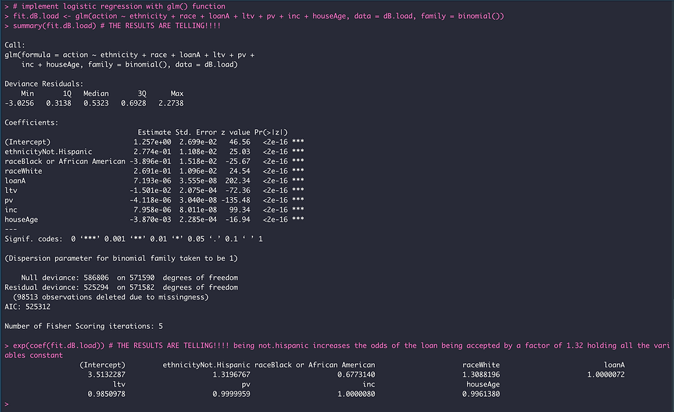
The results from logistic regression are shown above, in which the outcome being modeled is the log(odds) that action = 1 (in other words, the log odds that the action taken by the bank on the home loan applications is originated, that is accepted). When running summary(fit.dB.load) the p-values for the regression coefficients (column labeled Pr(>|z|) indicate that all variables in the dataset make a significant contribution to the equation that models the outcome variable (the action taken by the bank on the loan application).
When running (exp(coef(fit.dB.load) we are converting log odds to odd ratios and it is super interesting to note from the results above that only Not.Hispanic applicants (within the ethnicity variable) significantly contributes to the odds that the bank will originate/accept a home loan application! Specifically, the odds of a bank originating a home loan application when the ethnicity of the applicant is Not.Hispanic are increased by a factor of ~1.32 or 32% when holding all other variables constant.
A 95% confidence interval of the odds ratios can also be calculated using the confint() function, which facilitates the decision on evaluating how strong the evidence is that each variable has predictive value.
exp(cbind(Odds_ratio = coef(fit.dB.load), confint(fit.dB.load)))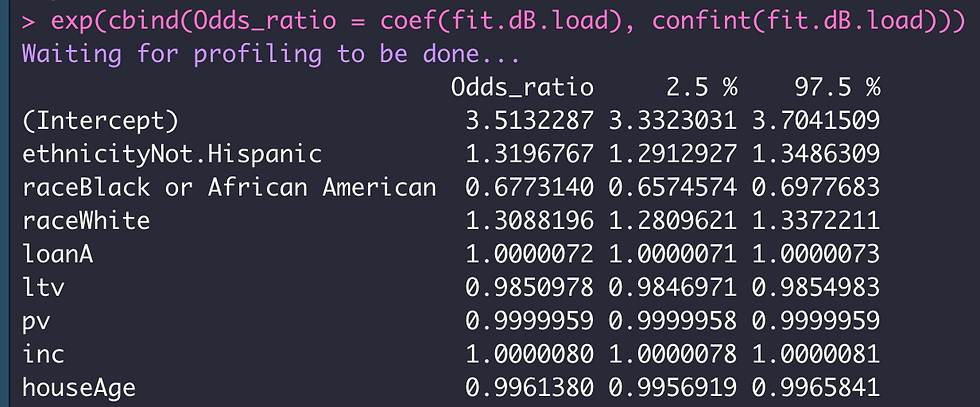
Based on the above, it can be seen that the odds ratio for the home loan being originated when the ethnicity of the applicant is Not.Hispanic is well within the confidence interval. Similarly, the odds ratios for a home loan origination are also within the confidence interval for the race variable, with the odds on loan origination increasing by a factor of ~1.31 or 31% when the applicant is White, and decreasing by a factor of ~ 1.48 (1 / 0.677 = 1.477 that is ~ 1.48) or 48% when the applicant is Black or African American, when holding all other variants constant.
When taking into account all the other variables in the dataset, it can be seen that their contribution to a decrease (ltv and houseAge) in the odds ratio of a home loan being originated is pretty small. The loan_to_value_ratio (ltv) and houseAge appears to affect the odds ratio of a home loan being originated with a one unit increase in ltv decreasing the odds of loan origination by a factor of 1.015 (1 / 0.985) or 1.5%, whereas houseAge decreasing the odds of loan origination by a factor of 1.004 (1 / 0.996) or 0.4%. Because the odds ratio for loanA and inc variables is 1 (the odds of a home loan being originated is equal to the odds of being denied), these two variables appears to have no effect in predicting the outcome on the action taken by the bank on the loan (origination vs denial).
I can evaluate the logistic regression model by plotting each observation against it predicted outcome and color the observations based on their actual values (Figure 1). Because most observations with actual 'denied' values (colored red in Figure 1) were predicted as having probabilities below 0.5; and most observations with actual 'originated' values (colored green in Figure 1) were predicted as having probabilities above 0.5, I can conclude the model made quite a satisfactory job!
# evaluate model by ploting each observation against it predicted outcome and color observations based on the actual value
predicted.action <- data.frame(
  probability.of.action = fit.dB.load$fitted.values,
  action = dB.load.reduced$action
)

predicted.action <- predicted.action[order(predicted.action$probability.of.action, decreasing = FALSE), ]
predicted.action$rank <- 1:nrow(predicted.action)
View(predicted.action) # observations in data frame are ordered accoring to the probability of the outcome variable, from 0 to 1

# plot model performance
ggplot(data = predicted.action, aes(x = rank, y = probability.of.action)) +
  geom_point(aes(color = action), alpha = 1, shape = 4, stroke = 2) +
  xlab("index") +
  ylab("predicted probability of home loan being accepted")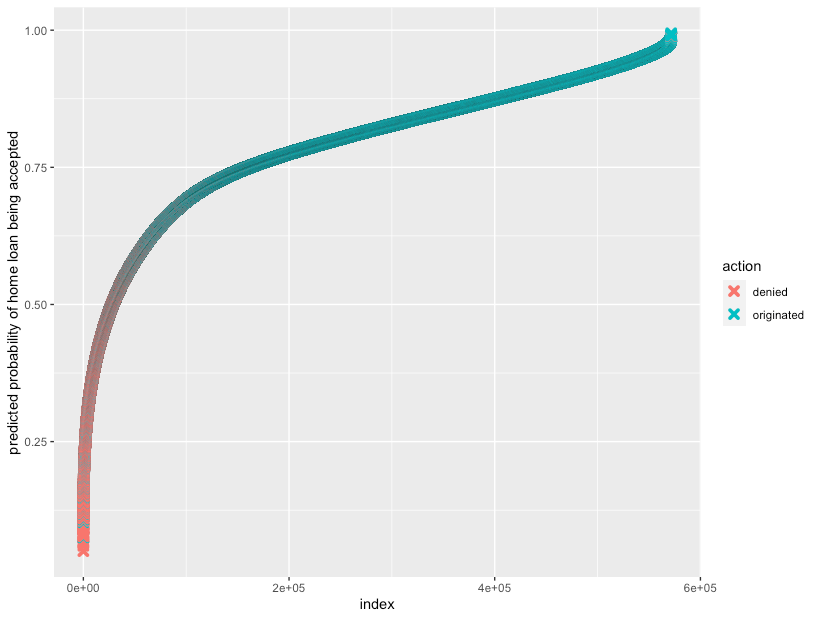
Figure 1. Plot to evaluate the performance of the logistic regression model described in this study. On the y-axis is the predicted probability of a home loan being accepted (1 = loan originated) while on the x-axis is each observation (loan application) ranked on predicted probabilities (from 0 to 1) . Observations are color coded according to their actual values in the dataset.
In summary, the logistic regression model was built taking into account 944 banks across New Jersey that processed 571,591 home loan applications during the years 2018, 2019 and 2020. The observation that the ethnicity and race of a home loan applicant is a relevant contributor in predicting the outcome of a loan being originated is the main result of this work, and support my previous findings that the latino community is disfavored by financial institutions when requesting loans to purchase a home.
This model could be used in the near future to predict the outcome of home loans originations with data collected in 2021 (still not available for public use). Also, I could implement a logistic regression model bank-by-bank to assess the contribution of an applicant's ethnicity in the probability of a home loan being originated. A bank-by-bank logistic regression model would have less predictive power since the number of observations is reduced compared to the number of observations when 944 banks combined is used.
I kept exploring the relationship between the ethnicity of a home loan applicant and the action taken by the bank on the loan application, this time by implementing a test of independence. My results from Chi-square test suggested that action taken by the bank and ethnicity are not independent variables.
# tests of independence (test independence of categorical variables)
# create contingency table action vs ethnicity
tB.load <- xtabs(~ action + ethnicity, data = dB.load)
tB.load

# chi-square
chisq.test(tB.load) # action and ethnicity are NOT independent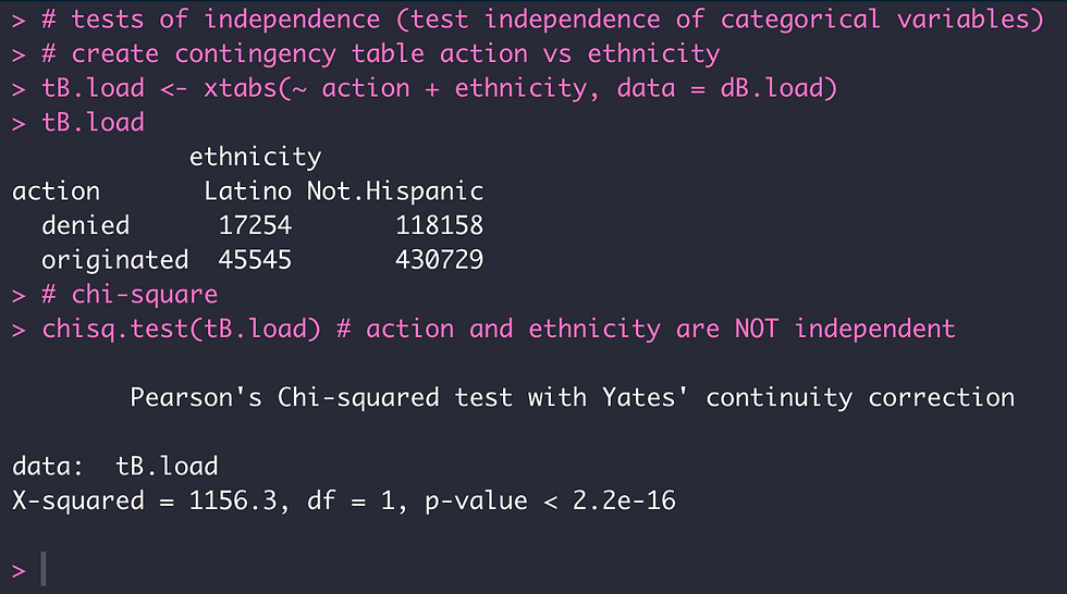
Mosaic plots allow for the graphical representation of contingency tables by drawing nested rectangular regions that are proportional to their cell frequency. Furthermore, mosaic plots allow for the use of color and shading to represent residuals from a fitted model (Pearson residuals from an independence test). I used a mosaic plot to visualize the relationship between action taken by the bank on home loan applications when the ethnicity of the applicant is Latino in comparison to Not.Hispanic (Figure 2).
# BLUE color indicates cross-classification between action and ethnicity occurs MORE OFTEN than expected
# RED color indicates cross-classification between action and ethnicity occurs LESS OFTEN than expected
mosaic(tB.load, shade = TRUE, las = 2)
Figure 2. Mosaic plot displaying cross classification that occur (a) more often than expected (indicated in blue color >> denied loan and Latino applicant, and originated loan and Not.Hispanic applicant); and (b) less often than expected (indicated in red color >> denied loan and Not.Hispanic applicant, and originated loan and Latino applicant), under the independence model respectively.
In summary, the results shown on Figure 2 indicate that Latino applicants are denied home loans more often than expected, and are granted home loans less often than expected.
Next, I created a contingency table that included the top 5 banks of New Jersey in terms of the total number of home loan applications processed in the three year period of study; and created a mosaic plot (Figure 3) that revealed the same pattern as in Figure 2 for a per-bank-basis.
# create contingency table for top 5 banks in New Jersey
bank.ID <- c(
  "KB1H1DSPRFMYMCUFXT09",
  "549300FGXN1K3HLB1R50",
  "B4TYDEB6GKMZO031MB27",
  "7H6GLXDRUGQFU57RNE97",
  "AD6GFRVSDT01YPT1CS68"
)

bank.name <- c(
  "WeFa",
  "RoMo",
  "BaAm",
  "JPM",
  "PNC"
)

# create a new data frame with top 5 financial institutions
dB.load.top5banks <- filter(dB.load, bank %in% bank.ID)
# replace leis with names
dB.load.top5banks$bank[dB.load.top5banks$bank %in% bank.ID] <- bank.name

describe(dB.load.top5banks[, c(6:11)])

# create contingency table
t_top5_banks <- xtabs(~ action + ethnicity + bank, data = dB.load.top5banks)
View(t_top5_banks)

# create mosaic plot
mosaic(~ bank + ethnicity + action, data = t_top5_banks, shade = TRUE, direction = c("v", "h", "v"))
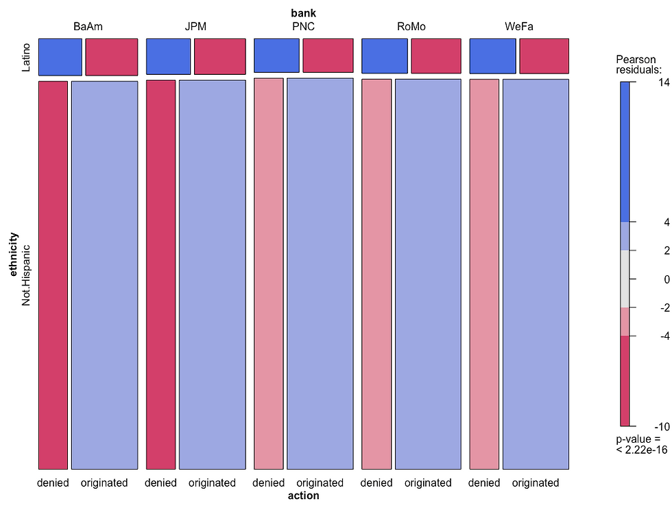
Figure 3. Mosaic plot displaying cross classification for the top 5 banks in New Jersey that occur (a) more often than expected and (b) less often than expected, under the independence model. Bank notation: Wells Fargo (WeFa), Rocket Mortgage (RoMo), Bank of America (BaAm), JPMorgan Chase (JPM), PNC Bank (PNC). This graphs clearly shows that Latino applicants are denied home loans more often than expected.
Question 2
What is the relation between interest_rate (ir) and loan_to_value_ratio (ltv) for Latino home loan applicants relative to Not.Hispanics?
In my previous work on Exploratory Data Analysis (EDA) I found that the median interest_rate (ir) on originated loans was higher for Latinos compared to Not.Hispanics. Since the HMDA dataset does not provide information on credit scores for each applicant, I look into the loan_to_value_ratio (ltv) for each application as an alternative. This was because ltv is an assessment of lending risk that banks look into prior to approving a mortgage. Loan applications with high ltv are considered riskier and thus, if the loans are approved, they have higher interest rates.
The loan_to_value_ratio is obtained by dividing the loan amount by the property value, expressed as percentage. Thus it is an indirect measurement of downpayment. When ltv is over 100% it means the market value of the property is less than the money owed on the loan.
The distribution of values for ltv and interest rate is shown in Figure 4. We can observe that loan originations from latinos display loan_to_value_ratio peaking at about a little over 95%, whereas Not.Hispanic loan originations display a peak at about 80% loan_to_value_ratio. Although differences in the distribution of loan_to_value_ratios between Latinos and Not.Hispanics might be a possible explanation for higher median interest rate for Latinos compared to Not.Hispanics; results obtained from a scatter plot of interest_rates vs loan_to_value_ratios shown in Figure 5 does not appear to support this notion.
# plot distribution of ltv for loan originations
ggplot(data = dB.originated, aes(x = ltv)) +
  geom_density(aes(color = ethnicity)) +
  scale_x_continuous(breaks=c(10, 20, 30, 40, 50, 60, 70, 80, 90, 100, 110, 120, 130)) +
  labs(title="Distribution of home loan originations according to loan_to_value_ratio", x="% loan to value ratio")

# plot distribution of interest rate for loan originations
ggplot(data = dB.originated, aes(x = ir)) +
  geom_density(aes(color = ethnicity)) +
  scale_x_continuous(breaks=c(1, 1.5, 2, 2.5, 3, 3.5, 4, 4.5, 5, 5.5, 6, 6.5, 7)) +
  labs(title="Distribution of home loan originations according to interest rate", x="% interest rate")
Figure 4. Kernel density plots displaying the distribution of loan_to_value_ratio (ltv) and interest_rate (ir) variables for Latino and Not.Hispanic loan originations, respectively. For each ethnic group, we should compare where the peak occurs (along the x-axis) for ltv and ir variables. Left graph: Whereas loan originations from Latinos display the biggest peak at about 95% for ltv, Not.Hispanics loan originations instead display the biggest peak at about 80%. Right graph: Whereas Latino loan originations display 4 similar peaks at interest rates between 2.75 and 4.75% approximately, Not.Hispanic loan originations display the biggest peak at almost 3%.
The relationship between interest rate and ltv for originated loans depending on the ethnicity of the applicant is shown in Figure 5. We can observe that the LOESS fit line associated with latino loan originations display higher values for interest rate compared to that of Not.Hispanics up to a loan_value_ratio of about 90%, when their LOESS fit lines merge, their confidence intervals overlap and values for interest rate increase above 4%.
# What is the relation between loan_to_value_ratio (ltv) and interest_rate (ir)?

# selected loans originated only (action == 1) because they all have interest rates
dB.originated <- dB.load[dB.load$action == "originated", ] # 534,692 observations & 11 variables
# remove missing values
dB.originated <- na.omit(dB.originated) # 449,279 observations & 11 variables

# plot ltv vs ir for originated loans
ggplot(data = dB.originated) +
  geom_jitter(aes(x = ltv, y = ir, shape = ethnicity)) +
  scale_shape_manual(values = c(1, 2)) +
  geom_smooth(aes(x = ltv, y = ir, color = ethnicity)) +
  scale_x_continuous(breaks=c(10, 20, 30, 40, 50, 60, 70, 80, 90, 100, 110, 120, 130)) +
  scale_y_continuous(breaks=c(1, 1.5, 2, 2.5, 3, 3.5, 4, 4.5, 5, 5.5, 6, 6.5, 7)) +
  labs(title="Loan to Value Ratio relative to Interest Rate", x="% loan to value ratio", y="% interest rate")
Figure 5. Scatter plot depicting loan_to_value_ratio relative to interest_rate, with a LOESS (locally weighted polynomial) fit line to facilitate in the identification of trend in the data. Observations (home loan applications that were originated) from Latino applicants are shown as circles (and the smoothing line in red color) whereas Not.Hispanic applicants are shown as triangles.
When looking at Figure 5, the surprising finding is that interest rates remained fairly constant for both ethnic groups of loan recipients (within the 3.5% to 4.25% interval) across a wide range of loan_to_value ratios up until 90%. Based on this, I am inclined to conclude that loan_to_value_ratios are not a good explanatory cause for higher interest rates observed in Latino loan originations relative to Not.Hispanics. My statement is further supported by results obtained from the implementation of partial correlation analysis; which shows a weak correlation between interest_rate and loan_to_value_ratio variables when controlling for loan_amount, property_value, income, and house_age.
# CORRELATION BETWEEN LTV AND IR

# correlation coefficients (to describe relationships among quantitative variables)
dB.originated.qvars <- scale(dB.originated[, c(6:11)]) # scale variables

cor(dB.originated.qvars) # interesting results

# are these correlations significant?
print(corr.test(dB.originated.qvars, use = "complete", ci = TRUE, minlength = 10), short = FALSE) # the above correlations are significant!
?corr.test()


# partial correlations
install.packages("ggm", dependencies = TRUE)
library(ggm)

colnames(dB.originated.qvars)
pcor(c(2, 3, 1, 4, 5, 6), cov(dB.originated.qvars)) # the correlation between variable 2 that is ltv (loan to property value ratio) ...
# ... relative to variable 3 that is ir (interest rate) i is 0.216, controlling for the influence of loanA, pv, inc and houseAge

# how about the above result for latino vs non latino originated loans? Do they show the same partial correlation between ltv and ir?
dB.oq.notHispanic <- dB.originated[dB.originated$ethnicity == "Not.Hispanic", ] # 406,488 observations
dB.oq.notHispanic <- dB.oq.notHispanic[, c(6:11)]
dB.oq.notHispanic <- scale(dB.oq.notHispanic)

colnames(dB.oq.notHispanic)
pcor(c(2, 3, 1, 4, 5, 6), cov(dB.oq.notHispanic)) # 0.22 is the correlation coefficient between ltv and ir for not.hispanic loan applications that were originated
corr.test(dB.oq.notHispanic, use = "complete")


# how about the above result for latino vs non latino originated loans? Do they show the same partial correlation between ltv and ir?
dB.oq.Latino <- dB.originated[dB.originated$ethnicity == "Latino", ]
dB.oq.Latino <- dB.oq.Latino[, c(6:11)]
dB.oq.Latino <- scale(dB.oq.Latino)

colnames(dB.oq.Latino)
pcor(c(2, 3, 1, 4, 5, 6), cov(dB.oq.Latino)) # 0.14 is the correlation coefficient between ltv and ir for latino loan applications that were originated
corr.test(dB.oq.Latino, use = "complete")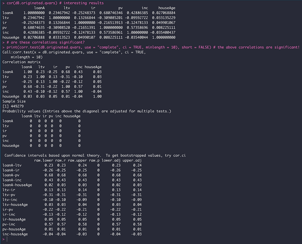
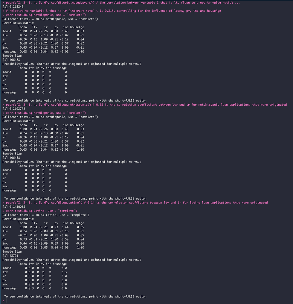
In summary, none of the variables I analyzed from the HMDA dataset can explain why Latinos home loan originations display a higher median value for interest rate compared to Not.Hispanics.
References
Robert I. Kabackoff (2015). R in Action: Data Analysis and Graphics with R (2nd Edition). Published by Manning, Shelter Island, NY 11964
Hefin I. Rhys (2020). Machine Learning with R, the tidyverse and mlr. Published by Manning, Shelter Island, NY 11964
Winston Chang (2019). R Graphics Cookbook: practical recipes for visualizing data. Published by O'Reilly, Sebastopol, CA 95472
Hadley Wickham & Garrett Grolemund (2017). R for Data Science: import, tidy, transform, visualize, and model data. Published by O'Reilly, Sebastopol, CA 95472


Comments